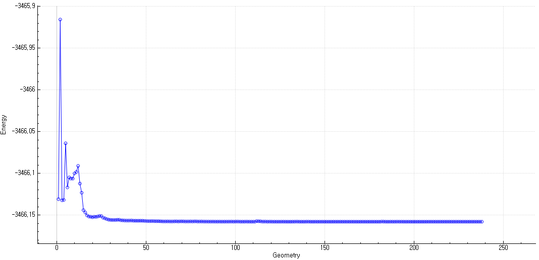
Hello. I have been trying to obtain a TS structure. Before running a TS optimization, to obtain an appropriate initial geometry of molecule, I run constrained optimization on the bond length with chemical intuition. The obtained results are shown below.
I thought the geometry with a B-O length of 2.2 A should be close to the TS structure, so I selected it as an the initial geometry. After running the TS optimization (JOBTYPE=TS), however, the final energy turned out to be almost the same as that of the previously optimized equilibrium geometry. In other words, the TS calculation seemed to behave like a normal geometry optimization. The resulting energy profile also resembled that of a standard optimization.
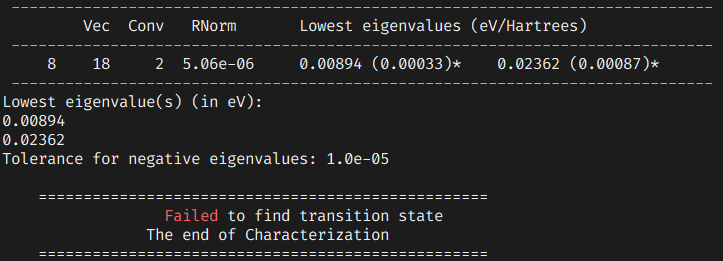
In addition, a Hessian-free characterization of stationary points indicated that this geometry corresponds to a local minimum, as it shows two positive eigenvalues.
Two suggestions:
(1) try the freezing string method (JOBTYPE = FSM) to get a better TS guess. Take the highest point along the string as your guess.
(2) For the proper TS search (JOBTYPE = TS), start with an exact Hessian. In the latest version of Q-Chem this is done automatically but not in older versions. For the latter, you need to do this as two separate jobs. The first one is JOBTYPE = FREQ (to compute the Hessian at your initial geometry, obtained e.g., from Freezing String). Subsequently, run JOBTYPE = TS and put GEOM_OPT_HESSIAN = READ into $rem.
Following your suggestion, I run a TS calculation including ‘GEOM_OPT_HESSIAN’ option and found a TS structure. The relevant output is shown below:
 ------------------------------------------------------------------------------
         Vec  Conv   RNorm       Lowest eigenvalues (eV/Hartrees)
 ------------------------------------------------------------------------------
     8    18     2  5.52e-06    -0.01523 (-0.00056)*    0.00181 (0.00007)*
 ------------------------------------------------------------------------------
Lowest eigenvalue(s) (in eV):
-0.01523
0.00181
Tolerance for negative eigenvalues: 1.0e-05

    ==================================================
        Successfully converged to a transition state
                The end of Characterization
    ==================================================
For this geometry, I run a frequency calculation to validate whether it corresponds to a true TS structure. However, there are 3 imaginary frequencies.
 **********************************************************************
 **                                                                  **
 **                       VIBRATIONAL ANALYSIS                       **
 **                       --------------------                       **
 **                                                                  **
 **        VIBRATIONAL FREQUENCIES (CM**-1) AND NORMAL MODES         **
 **     FORCE CONSTANTS (mDYN/ANGSTROM) AND REDUCED MASSES (AMU)     **
 **                  INFRARED INTENSITIES (KM/MOL)                   **
 **                                                                  **
 **********************************************************************


 Mode:                 1                      2                      3
 Frequency:       -91.66                 -32.00                 -17.25
 Force Cnst:      0.0370                 0.0042                 0.0011
 Red. Mass:       7.4747                 7.0106                 6.2558
 IR Active:          YES                    YES                    YES
 IR Intens:        7.991                  1.492                  0.978
 Raman Active:       YES                    YES                    YES
Could you explain why the obtained TS structure yields more than one imaginary frequency? The only minor difference between the two calculations is the choice of SCF algorithm: the former used DIIS, while the latter used DIIS_GDM.
This means you have several normal modes where the potential energy surface curves downward, i.e., a higher-order saddle point. You should visualize the modes in question because several of the imaginary frequencies are very small. That may suggest a way to displace the structure off of a higher-order saddle point. Alternatively (or in addition), try tightening the geometry optimization stopping criteria, say:
in $rem, which is 2x tighter than the default criteria. The smallness of the 32i and 17i cm^(-1) frequencies suggests a flat potential surface where the optimization may have stopped before reaching a proper 1st-order saddle point.