Overview
In an approximate photoelectron spectroscopy simulation, the norm square of Dyson orbitals are usually taken as a quick estimation of the ionization intensities. However, for quantitative calculations of total and differential ionization cross sections, the photoelectron matrix element should be calculated and evaluating both Dyson orbitals and the wave functions of the leaving photoelectrons is necessary. Q-Chem can calculate Dyson orbitals at the EOM-CC level of theory, which makes calculating absolute photodetachment/photoionization cross sections, photoelectron angular distributions (PADs), and anisotropy parameters (β) using the ezDyson program package possible. In addition, the Franck-Condon factors between the vibrational states of the ionized and neutral species can be calculated by another program package ezSpectrum, therefore the vibrational structures of photoelectron spectroscopy can be studied.
In the following we will illustrate how to simulate photoelectron spectroscopy using Q-Chem with ezDyson and ezSpectrum step-by-step.
Quantum Chemistry Calculations with Q-Chem
Before we run ezDyson and ezSpectrum, Q-Chem calculations need to be carried out in order to produce the necessary Dyson orbitals and other relevant information. The following is an example qchem input file:
Example 1. An EOM-IP-CCSD calculation of a methanol molecule. Geometry optimized at the 𝜔B97X-D/aug-cc-pVTZ level of theory (comments after the symbol “!”).
$molecule
0 1
C         0.660492       -0.036257    0.000000
O        -0.742798     0.118380    0.000000
H         1.019207      -0.559731      -0.891530
H         1.019207       -0.559731    0.891530
H         1.087065     0.964343    0.000000
H        -1.152635       -0.745352    0.000000
$end
$rem
jobtype = SP
correlation = CCSD
BASIS = aug-cc-pVTZ
purecart = 111        ! Required for ezDyson to know if pure or cartesian functions are used.
scf_convergence = 7
MAX_SCF_CYCLES = 150
ip_states = [1,1]    ! Requests Dyson orbital for states with specific symmetries
ccman2 = true        ! Invoke the ccman2 code
cc_trans_prop = true    ! Request the transitions between all EOM states and the reference state
cc_do_dyson = true    ! Calculate Dyson orbitals
cc_t_conv = 7
eom_davidson_convergence = 6
print_general_basis = true    ! Prints basis set information in output, needed for ezDyson
molden_format = 1    ! Print out Dyson orbitals in the MOLDEN format, needed for visualization
$end
After the calculation is done, the Dyson orbitals can be visualized by IQmol, the graphical frontend software of Q-Chem. Just open the qchem output file with IQmol, and select “Dyson orbital” from ’Surfaces’ on the left side panel; then select the transition for which the Dyson orbital will be plotted. An example calculated Dyson orbital of methanol in IQmol is shown in the following figure:
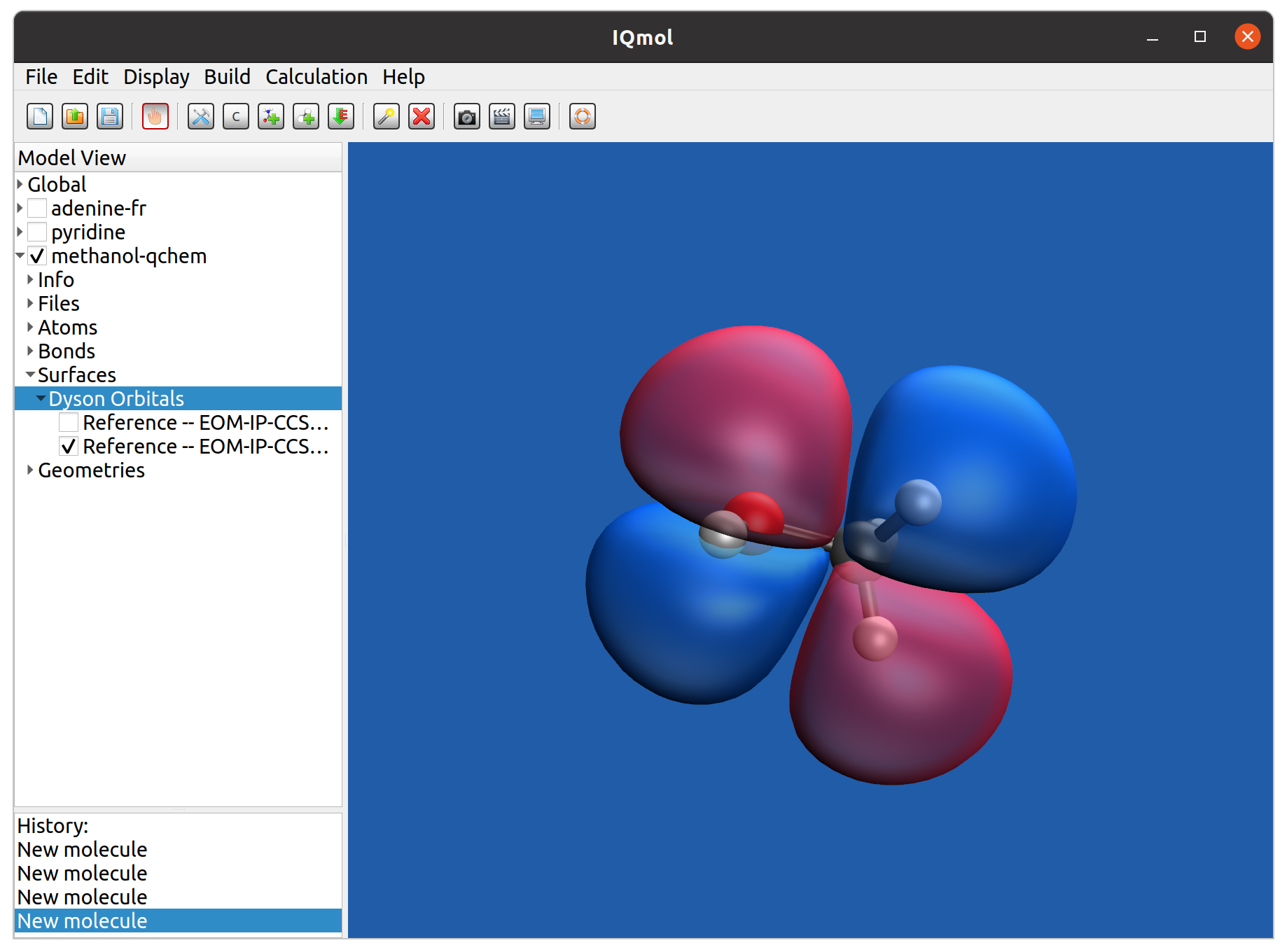
Fig. 1: Visualization of Dyson orbitals with IQmol.
Photoionization Cross Section Calculation with ezDyson
- Obtain ezDyson
Download the current version of ezDyson from the link: http://iopenshell.usc.edu/downloads/ezdyson/ezdyson.v4.tar.gz
and run (under Linux)
tar -zvxf ezdyson.v4.tar.gz
to extract the files. Usually the pre-compiled executable (exedys) can run under Linux. If not, please copy the makefiles for different platforms provided in the main directory (copy the “mk” file for the proper platform into makefile), and run:
make clean
then
make
to compile the code and generate the executable. For more details about the package, please refer to the manual from the link: http://iopenshell.usc.edu/downloads/ezdyson/ezDysonManual.pdf
- Generate ezDyson input file from qchem output file.
Suppose the qchem output file in the last section is “methanol-qchem.out”, and the path to the extracted ezDyson directory is PATHDYSON, one can run the command:
PATHDYSON/ezDyson/xmlsamples/makexml_script/make_xml_IPEA.py methanol-ezdy.xml methanol-qchem.out
Here the python script make_xml_IPEA.py generates the ezDyson input file methanol-ezdy.xml from the qchem output file.
- Modify the ezDyson input file if necessary.
The head part of the ezDyson input file methanol-ezdy.xml is as follows:
Example 2. The head of ezDyson input file of methanol (notes after the symbol “!”) .
<?xml version="1.0" encoding="ISO-8859-1"?>
<root
  job = "dyson"
  >

<geometry
 n_of_atoms="6"
 text = "
      C       0.6610636725        -0.0210744946    -0.0000000000
      O      -0.7435042327        0.1214892640      0.0000000000
      H       1.0242669977        -0.5414443867    -0.8915300000
      H       1.0242669977        -0.5414443867      0.8915300000
      H       1.0790162890         0.9831568008    -0.0000000000
      H      -1.1458984577       -0.7457351718      0.0000000000
  "
/>

<free_electron
   l_max = "5" ! l_max=5 is usually enough for low energy ionization. See ezDyson manual.
   charge_of_ionized_core = "0" > ! 0 is plane wave, 1 is coulomb wave, you can also use <1 as effective charge.
     <k_grid n_points="11" min="0.01" max="1.01" />     ! Kinetic energies for which to compute cross sections, in eV. Should be changed if necessary.
</free_electron>

<averaging
   method= "avg" ! How to average over molecular orientations. Avg is faster as long as l_max is converged.
   method_possible_values="noavg, avg, num" >
</averaging>

<laser
   ionization_energy = "10.84" > ! Ionization energy of the molecule. Needs to be specified. Here the number “10.84” is for methanol.
   <laser_polarization x="0.0" y="0.0" z="1.0" /> ! For “avg”, this does nothing. Only for “noavg”.
</laser>

<lab_xyz_grid> ! Numerical integration grid. This is ok if the integrate norm ~1.
 <axis n_points="201" min="-10.0" max="10.0" />
 <axis n_points="201" min="-10.0" max="10.0" />
 <axis n_points="201" min="-10.0" max="10.0" />
</lab_xyz_grid>
……
The other parts of the .xml file just copies information from the qchem output file such as the basis functions and Dyson orbitals, which can be left untouched.
- Run ezDyson.
Once the .xml file is well prepared, you can run ezDyson with the command: PATHDYSON/ezDyson/exedys methanol-ezdy.xml > methanol-ezdy.out
- Result analysis.
In the output file “methanol-ezdy.out” before the content copied from the .xml input file, one can see a summary of the calculated ionization cross sections and anisotropy:
Example 3. Summary of the calculated ionization cross sections and anisotropy of methanol.
E=IE+E_k,eV   Sigma_par     Sigma_perp    Sigma_tot     beta
10.850000      0.000012      0.000009      0.000125      0.190750
10.950000      0.000396      0.000306      0.004223      0.177615
11.050000      0.000990      0.000789      0.010759      0.156109
11.150000      0.001683      0.001385      0.018654      0.134058
11.250000      0.002427      0.002061      0.027432      0.111715
11.350000      0.003189      0.002797      0.036794      0.089172
11.450000      0.003949      0.003580      0.046529      0.066489
11.550000      0.004691      0.004396      0.056480      0.043714
11.650000      0.005405      0.005239      0.066529      0.020886
11.750000      0.006082      0.006100      0.076580       -0.001958
11.850000      0.006718      0.006974      0.086561       -0.024785
Plotting the E (first column) vs. Sigma_tot, you get the “photoionization spectrum”. Plotting E vs. beta you get the information on how the anisotropy parameter varies with energy. PADs are printed in a separate file named pad.dat.
Franck-Condon Factor (FCF) Calculation with ezSpectrum
- Run Q-Chem to obtain the optimized geometries and vibrational frequencies and normal mode vectors of both the ground and ionized states.
The example Q-Chem input files for the geometry optimization and frequency calculations of the ionized state of methanol are as the following:
Example 4. Q-Chem input files for the geometry optimization and frequency calculations of the ionized state of methanol.
$comment
Geometry optimization
$end

$molecule
1 2
 C         0.660492       -0.036257    0.000000
 O       -0.742798     0.118380    0.000000
 H         1.019207       -0.559731      -0.891530
 H         1.019207       -0.559731    0.891530
 H         1.087065     0.964343    0.000000
 H       -1.152635       -0.745352    0.000000
$end

$rem
   BASIS  =  aug-cc-pVTZ
   JOB_TYPE  =  Optimization
   exchange  =  omegaB97X-D
   SCF_CONVERGENCE  =  8
   sym_ignore = true
   symmetry = false
$end

*************************************************************************************************************
$comment
Geometry optimization
$end

$molecule
1 2
 C         0.6510503166         0.0426377405     0.0000000201
 O       -0.6979023816         0.1143406096       -0.0000000149
 H         0.9951302666       -0.6240943420       -0.8380349100
 H         0.9951302927       -0.6240943394     0.8380349133
 H         1.0882097264         1.0330700697       -0.0000000061
 H       -1.1410802206       -0.7602077383     0.0000000000
$end

$rem
   BASIS  =  aug-cc-pVTZ
   JOB_TYPE  =  Freq
   exchange  =  omegaB97X-D
   MAX_SCF_CYCLES  =  150
   sym_ignore = true
   symmetry = false
   threads 4
   mem_static = 2000
   cc_memory = 14000
$end
- Obtain ezSpectrum
Download the current version of ezSpectrum from the link: http://iopenshell.usc.edu/downloads/ezSpectrum.v3.0.tar.gz
and run (under Linux)
tar -zvxf ezSpectrum.v3.0.tar.gz
to extract the files. Usually the pre-compiled executable (ezSpectrum.64) can run under Linux.
- Prepare the ezSpectrum input file.
Copy the qchem output files of the frequency calculations of both the ground and ionized states of methanol into your working directory. Suppose these files are called “methanol-S0.out” and “methanol-D1.out”. Suppose the path to the ezSpectrum directory is PATHSPEC, copy two file from the ezSpectrum directory to your working directory by running the commands:
cp PATHSPEC/ezSpectrum/atomicMasses.xml .
cp PATHSPEC/ezSpectrum/make_xml.py .
Then run the python script make_xml.py to generate the input methanol-ezSpec.xml file for ezSpectrum:
./make_xml.py methanol-ezSpec.xml methanol-S0.out methanol-D1.out
Note: do not change the order of the two qchem output files in the command above.
- Modify the .xml input file if necessary.
Open the methanol-ezSpec.xml file and change the temperature on the fifth line from 300 to 0. Then change the ionization potential (ip), which is right under the “<target_state>” section of the xml input file. By default, the xml file has 1; change the 1 to 10.84, the actual experimental IP for the methanol.
- Run ezSpectrum.
Run the command:
PATHSPEC/ezSpectrum/ezSpectrum.64 methanol-ezSpec.xml > methanol-ezSpec.out
- Use the script xsecFCF to combine the results of ezDyson and ezSpectrum and get the photoelectron data for plotting.
The script xsecFCF can be found in PATHDYSON/xmlsamples/xsecFCF. It requires two files called FCFs.dat and xsec.dat. The first file can be copied from an output file from the ezSpectrum calculation, usually called filename.xml.spectrum_parallel or filename.xml.spectrum_duschinsky (depending on the options used in ezSpectrum). This file needs to be modified by adding only one line in the beginning of the file indicating the total number of FCF transitions included in the file. The second file, xsec.dat, is just a segment copied from the ezDyson output from the section titled “Total cross-section / E (in a.u.) vs. Ek (in eV)”, with again one additional line indicating the number of energies for which cross sections were computed. Note that for ezSpectrum, ionization energies (first column) are reported as negative numbers, so you need to convert them all to positive values first for the script to work correctly. Put FCFs.dat and xsec.dat into the same folder as xsecFCF and run the script:
./xsecFCF > xsecFCF.out
In the end of the output file xsecFCF.out you will see the result summary:
Example 5. Photoionization cross sections with Franck-Condon factors of methanol.
Ionization energy: 10.84000
cross-sections after accounting for Franck-Condon factors:
E, eV     xsec, a.u.
10.85000  0.00003
10.95000  0.00093
11.05000  0.00330
11.15000  0.00722
11.25000  0.01267
11.35000  0.01938
11.45000  0.02703
11.55000  0.03538
11.65000  0.04420
11.75000  0.05330
11.85000  0.06255
The results can be shown in the following picture:

Fig. 1: Absolute cross sections for photoionization of methanol with different screened nuclear charges (Z). Adapted from J. Phys. Chem. Lett., 6, 4532 (2015).