Simulating Vibronic and Resonance Raman Spectroscopy Using the VIBRONIC module of Q-Chem

[yzhang]

Understanding the vibrational fine structure of electronic absorption and emission (vibronic) and vibrational resonance Raman spectroscopy plays an important role in characterizing molecular and electronic structure of molecules. In principle one needs the information of vibrational states on top of different electronic states to determine the corresponding spectroscopy signals.

Q-Chem provides a module VIBRONIC implemented by Xunkun Huang, Huili Ma and Wanzhen Liang [1-3] to simulate vibrationally resolved one-photon absorption (OPA) and one-photon emission (OPE) as well as resonance Raman spectroscopy (RRS). The key quantity to determine OPA, OPE and RRS signals is the polarizability tensor, which is usually in the form of sum-over-states (SOS). Evaluating SOS expressions could make the simulation costly. In the VIBRONIC module, the SOS expression is transformed into the time domain and the polarizability tensor is calculated through Fourier transform of the Green’s function (propagator) in the time domain. Currently the VIBRONIC module is available in TDHF, CIS and TDDFT calculations.

Since for these spectroscopies (OPA, OPE and RRS), two electronic states (the ground state g and the excited state e) are involved, the signal simulation usually consists of two steps (one step for each electronic state) except in the VG model. Available theoretical models at different levels of approximation include:

1. FC1 (available for OPA, OPE and RRS simulation). The Franck-Condon (FC) approximation is employed. In this model both ground and excited state geometries are required, but on the ground state vibrational frequencies are necessary. The excited state vibrational frequencies are assumed the same as the ground state vibrational frequencies and the Duschinsky rotation effect is neglected.
2. FC2 (available for OPA, OPE and RRS simulation). The Franck-Condon approximation is employed. Optimized geometries and vibrational frequencies are required both for the ground and excited states. Duschinsky rotation is included.
3. FCHT (available for OPA, OPE and RRS simulation). Both the FC and Hertzberg-Teller (HT) terms in the transition dipole moment Taylor expansion are considered. Optimized geometries and vibrational frequencies are required both for the ground and excited states. Duschinsky rotation is included.
4. VG (available for OPA and RRS simulation). The vertical gradient (VG) approximation is employed. Only ground state optimized geometry and vibrational frequencies are required and so the simulation can be finished in one step. The excited state vibrational frequencies are assumed the same as the ground state vibrational frequencies and the Duschinsky rotation effect is neglected. The displacement vector between the ground and excited state vibrational normal modes are approximately calculated from the excited state energy gradients (available in excited state force calculations). HT terms are also neglected.

The following are examples of vibronic spectroscopy and RRS simulations. Please make sure both steps of calculations should access the same scratch directory, as the vibronic parameters saved from the previous step should be available for the later step. In order to do so, one can either run a two-step job using the “@@@” delimiter, or run two separated calculations with the same predefined scratch directory name. For example, running the following commands:

qchem  input_file_for_state_1  output_file_for_state_1  your_scratch_directory_name
qchem  input_file_for_state_2  output_file_for_state_2  your_scratch_directory_name

The vibronic spectra simulation must run after the vibronic parameters are saved (see the examples below). In all simulations the $rem variable SYM_IGNORE must be set to TRUE in order to prevent the molecular geometry being transformed to the standard orientation. Q-Chem provides two $rem variables and one input section to control vibronic spectra simulation. For details please refer to the manual.

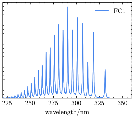
Example 1. Simulating the OPA signals of formaldehyde with TDDFT and the FC1 model.
Q-Chem Input for step 1: excited state (S1) geometry optimization (comments are put after the “!” sign and should be removed in case qchem does not run properly)

$molecule
0 1
 O                  0.003000000    0.00000000    0.68241638
 C                  0.020000000    0.00000000    -0.57598362
 H                   -0.030000000    0.92664718    -1.11098362
 H                  0.004000000  -0.92664718   -1.11098362
$end

$rem
  jobtype opt
  method b3lyp
  basis def2-TZVP
  cis_state_deriv 1    ! excited state no. 1
  cis_singlets true
  cis_triplets false
  cis_n_roots 10
  sym_ignore true    ! this must be set to TRUE
  save_vibronic_params true    ! save the vibronic parameter for later use
$end

Q-Chem Input for step 2: ground state (S0) geometry optimization and frequency and OPA simulation (comments are put after the “!” sign and should be removed in case qchem does not run properly)

$molecule
0 1
 O                  0.00000000    0.00000000    0.68241638
 C                  0.00000000    0.00000000   -0.57598362
 H                   -0.00000000    0.92664718   -1.11098362
 H                  0.00000000   -0.92664718    -1.11098362
$end

$rem
  jobtype opt
  method b3lyp
  basis def2-TZVP
  sym_ignore true
$end

@@@

$molecule
read
$end

$rem
  jobtype freq
  method b3lyp
  basis def2-TZVP
  sym_ignore true
  vibronic_spectra 1    ! simulating OPA
$end

$vibronic    ! the input section to control vibronic spectra simulation
  model 1    ! using the FC model
  freq_range 20000. 60000. 10.    ! simulation frequency range parameters in cm-1.
  time_range 1.0000000 40000    ! time step size in a. u. and no. of steps.
  damping 40.00000            ! damping factor in cm-1.
$end

Note: in order to break the symmetry, the starting geometry in step 1 is slightly different from that in step 2. In addition, excited state geometry optimization could be subtle. One should make sure the target excited state does not change its character (e. g., the order of all calculated excited states has not changed) during the geometry optimization process.

The resulted OPA signals are saved in a file named “abs_spectra.dat” and can be plotted as

The scratch files used in the OPA signal calculation can be found in a directory called “your_output_file_name.files” under the same directory as where the output file is generated.

Example 2. Simulating the OPE signals of formaldehyde with TDDFT and the FC2 model.
Q-Chem Input for step 1: excited state (D1) geometry optimization and frequency calculation (comments are put after the “!” sign and should be removed in case qchem does not run properly)

$molecule
0 2
 C         1.4840482200        0.0000338155        0.0000000000
 C         0.7160497031        0.0000524901       -1.2119311870
 C        -0.7159596058    0.0000542629       -1.2126930961
 C        -1.4043236629    0.0000543088        0.0000000000
 C        -0.7159596058    0.0000542629        1.2126930961
 C         0.7160497031        0.0000524901        1.2119311870
 C         2.8748450131        0.0000120580        0.0000000000
 H         1.2370230923        0.0000896598       -2.1693859212
 H        -1.2717579173    0.0000412967       -2.1497435961
 H        -1.2717579173    0.0000412967        2.1497435961
 H         1.2370230923        0.0000896598        2.1693859212
 H         3.4346492051        0.0000003003       -0.9330758768
 H         3.4346492051        0.0000003003        0.9330758768
 F        -2.7508602624    0.0000394216        0.0000000000
$end
$rem
  jobtype opt
  method b3lyp
  basis def2-SVP
  cis_state_deriv 1
  cis_singlets true
  cis_triplets false
  cis_n_roots 10
  sym_ignore true
$end

@@@

$molecule
read
$end

$rem
  jobtype freq
  method b3lyp
  basis def2-SVP
  cis_state_deriv 1
  cis_singlets true
  cis_triplets false
  cis_n_roots 10
  sym_ignore true
  save_vibronic_params true    ! save the vibronic parameter for later use
$end

Q-Chem Input for step 2: ground state (D0) geometry optimization and frequency calculation and OPE simulation (comments are put after the “!” sign and should be removed in case qchem does not run properly)

$molecule
0 2
 C         1.4566183503        0.0129101640        0.0000000000
 C         0.7101644786        0.0081907583       -1.2185833193
 C        -0.6759989496       -0.0007979055       -1.2214548662
 C        -1.3520058015       -0.0052290244    0.0000000000
 C        -0.6759989496       -0.0007979055    1.2214548662
 C         0.7101644786        0.0081907583        1.2185833193
 C         2.8635151754        0.0218512897        0.0000000000
 H         1.2491028005        0.0118050196       -2.1666316459
 H        -1.2458865325       -0.0044564748       -2.1504521674
 H        -1.2458865325       -0.0044564748    2.1504521674
 H         1.2491028005        0.0118050196        2.1666316459
 H         3.4244334505        0.0256959046       -0.9338584025
 H         3.4244334505        0.0256959046        0.9338584025
 F        -2.7015919823       -0.0141481171    0.0000000000
$end

$rem
  jobtype opt
  method b3lyp
  basis def2-SVP
  sym_ignore true
$end

@@@

$molecule
read
$end

$rem
  jobtype freq
  method b3lyp
  basis def2-SVP
  sym_ignore true
  vibronic_spectra 2    ! simulating OPE
$end

$vibronic
  model 1    ! using the FC model
  temperature 0.    ! simulation temperature in K.
  freq_range 1. 40000. 10.
  time_range 1. 40000
  damping 20.
$end

Note: One should confirm that the excited state geometry really is at a local minimum by the calculated vibrational frequencies.

The resulted OPE signals are saved in a file named “emiss_spectra.dat” and can be plotted as

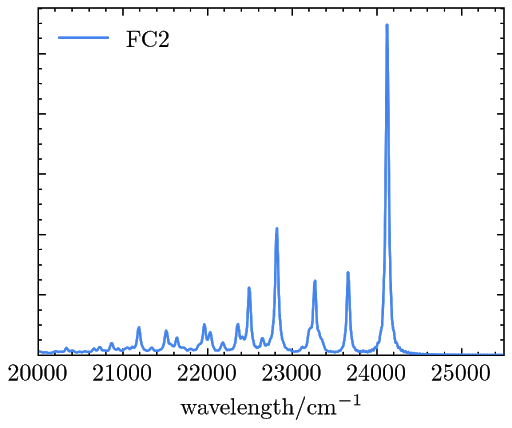
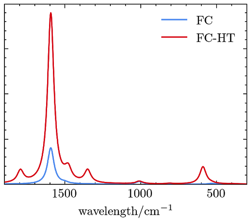
Example 3. Simulating the RRS signals of phenoxyl with TDDFT and the FCHT model.
Q-Chem Input for step 1: excited state (D3) geometry optimization and frequency calculation (comments are put after the “!” sign and should be removed in case qchem does not run properly)

$molecule
0 2
 C         0.0000000000        1.2502862746       -1.0797670264
 C         0.0000000000        0.0002405852       -1.8221303158
 C         0.0000000000       -1.2495301785       -1.0796765524
 C         0.0000000000       -1.2430453219    0.2902274202
 C         0.0000000000       -0.0000629947    1.0386563677
 C         0.0000000000        1.2431472440        0.2901098645
 H         0.0000000000        2.1927860816       -1.6322129361
 H         0.0000000000       -0.0006440427       -2.9122962915
 H         0.0000000000       -2.1925083031       -1.6316088409
 H         0.0000000000       -2.1692045915    0.8680624075
 H         0.0000000000        2.1689368505        0.8682996003
 O         0.0000000000       -0.0004016035    2.3373913028
$end

$rem
  jobtype opt
  method b3lyp
  basis def2-SVP
cis_state_deriv 3    ! excited state no. 3
  cis_singlets true
  cis_triplets false
  cis_n_roots 10
  sym_ignore true
$end

@@@

$molecule
read
$end

$rem
  jobtype freq
  method b3lyp
  basis def2-SVP
  cis_state_deriv 3
  cis_singlets true
  cis_triplets false
  cis_n_roots 10
  sym_ignore true
  save_vibronic_params true    ! save the vibronic parameter for later use
$end

Q-Chem Input for step 2: ground state (D0) geometry optimization and frequency calculation and RRS simulation (comments are put after the “!” sign and should be removed in case qchem does not run properly)

$molecule
0 2
 C         0.0000000000        1.2267763413       -1.0873977233
 C         0.0000000000        0.0003129951       -1.7857718635
 C         0.0000000000       -1.2259217607       -1.0872681918
 C         0.0000000000       -1.2399944954    0.2921692642
 C         0.0000000000       -0.0001222804    1.0534497246
 C         0.0000000000        1.2400986319        0.2919975911
 H         0.0000000000        2.1644176592       -1.6487443117
 H         0.0000000000       -0.0006702414       -2.8784475224
 H         0.0000000000       -2.1641202680       -1.6480392688
 H         0.0000000000       -2.1702849650    0.8642269804
 H         0.0000000000        2.1700059139        0.8643911139
 O         0.0000000000       -0.0004975303    2.3044892072
$end

$rem
  jobtype opt
  method b3lyp
  basis def2-SVP
  sym_ignore true
$end

@@@

$molecule
read
$end

$rem
  jobtype freq
  method b3lyp
  basis def2-SVP
  sym_ignore true
  vibronic_spectra 3    ! simulating RRS
$end

$vibronic
  model 2    ! using the FCHT model
  temperature 0.
  freq_range 1. 4000. 1.
  time_range 1. 40000
  damping 100.
  epsilon 25.    ! line broadening factor for RRS, in cm-1.
$end

The resulted RRS signals are saved in a file named “rrs_spectra.dat” and can be plotted as

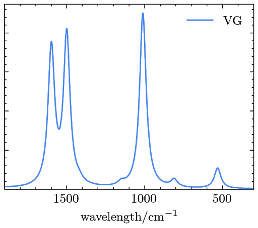
Example 4. Simulating the RRS signals of phenoxyl with TDDFT and the VG model.
Q-Chem Input: ground state (D0) geometry optimization and frequency calculation and excited state force calculation (comments are put after the “!” sign and should be removed in case qchem does not run properly)

$molecule
0 2
 C         0.0000000000        1.2267763413       -1.0873977233
 C         0.0000000000        0.0003129951       -1.7857718635
 C         0.0000000000       -1.2259217607       -1.0872681918
 C         0.0000000000       -1.2399944954    0.2921692642
 C         0.0000000000       -0.0001222804    1.0534497246
 C         0.0000000000        1.2400986319        0.2919975911
 H         0.0000000000        2.1644176592       -1.6487443117
 H         0.0000000000       -0.0006702414       -2.8784475224
 H         0.0000000000       -2.1641202680       -1.6480392688
 H         0.0000000000       -2.1702849650    0.8642269804
 H         0.0000000000        2.1700059139        0.8643911139
 O         0.0000000000       -0.0004975303    2.3044892072
$end

$rem
  jobtype opt
  method b3lyp
  basis def2-SVP
  sym_ignore true
$end

@@@

$molecule
read
$end

$rem
  jobtype force        ! excited state force calculation
  method b3lyp
  basis def2-SVP
  cis_state_deriv 3
  cis_singlets true
  cis_triplets false
  cis_n_roots 10
  sym_ignore true
  save_vibronic_params true    ! save the vibronic parameter for later use
$end

@@@

$molecule
read
$end

$rem
  jobtype freq        ! ground state frequency calculation
  method b3lyp
  basis def2-SVP
  sym_ignore true
  vibronic_spectra 3    ! simulating RRS
$end

$vibronic
  model 3    ! using the VG model
  temperature 0.
  freq_range 1. 4000. 1.
  time_range 1. 40000
  damping 100.
  epsilon 25.
$end

The resulted RRS signals are saved in a file named “rrs_spectra.dat” and can be plotted as

Reference:
[1] Wanzhen Liang et al., J. Phys. Chem. B, 110, 9908 (2006).
[2] Huili Ma, Jie Liu and Wanzhen Liang, J. Chem. Theory Comput., 8, 4474 (2012).
[3] Wanzhen Liang, Huili Ma, Hang Zang and Chuanxiang Ye, Int. J. Quantum Chem., 115, 550 (2015).

[AnnaKrylov]

FCFs can also be computed by a post-processing code ezFCF, which provides more flexibility in terms of underlying electronic structure method:

How to compute Franck-Condon factors

Franck-Condon factors (FCFs) are needed for modeling vibrational progression in electronic spectra. Most often FCFs are needed for computing UV-VIS and photoelectron spectra, but they also enter other workflows (such as ET rate calculations). FCFs can be computed using stand-alone ezSpectrum code: http://iopenshell.usc.edu/downloads/ which smoothly interacts with Q-Chem’s outputs. The details are described in ezSpectrum manual: http://iopenshell.usc.edu/downloads/manual.pdf

The software is described in this paper:
https://onlinelibrary.wiley.com/doi/epdf/10.1002/wcms.1546

[Salbej]

Greetings,
Do you have any recommandations of how to chose the dampind and epsilon factors in order to get high resolution spectrum for example?

Thanks

[yzhang]

I’m contacting the author of this vibronic module for an answer.

[yzhang]

The following is the reply from Prof. WanZhen Liang:

“These two quantities are closely related to the spectral resolution and are determined by the excited-state lifetime which is dependent on the molecule itself and its environment. You may take the same value for the two quantities in your calculation. Usually the smaller the higher resolution. However, if you input a smaller value, you have to calculate the propagation matrix for longer time because we adopt the time-dependent approach to calculate the RRS spectra. We firstly calculate the spectral cross sections in time-domain then made the Fourier transformation to them back to the frequency domain.
If the experimental spectra or molecular excited-state lifetime are available，you may take the values based on the experimental data.”

[liangwz_xmu]

These two quantities are closely related to the spectral resolution and are determined by the excited-state lifetime which is dependent on the molecule itself and its environment. You may take the same value for the two quantities in your calculation. Usually the smaller the higher resolution. However, if you input a smaller value, you have to calculate the propagation matrix for longer time because we adopt the time-dependent approach to calculate the RRS spectra. We firstly calculate the spectral cross sections in time-domain then made the Fourier transformation to them back to the frequency domain.

If the experimental spectra or molecular excited-state lifetime are available，you may take the values based on the experimental data.